GANs for Unsupervised Anomaly Detection

Author: Stephen Welch

In this article we’ll discuss why unsupervised learning is so compelling, especially in industries like manufacturing. We’ll build and train a Generative Adversarial Network (GAN) on a manufacturing dataset, create an anomaly detection algorithm using our trained GAN, and explore its performance.

The Dream of Unsupervised Learning

It’s difficult to fully grasp the scale of modern manufacturing. This year manufacturers will churn out over 50 billion square feet of carpet, more than 100 quintillion transistors, and in excess of one billion toothbrushes. That’s over 1900 new toothbrushes every second. Now, let’s say you work for one of these manufacturers, and it’s your job to ensure that each product that reaches your customers is of good quality.

How do you do it? You could hire an army of inspectors to manually inspect each item, but as you can imagine this can bring huge training and labor challenges, and repeating a task like this day in and day out is just not something we humans are terribly good at.

For the last 30 years or so, a relatively common approach in modern manufacturing is to automate inspection using cameras and computers. Snap a picture of each product, process the pixels in that image using an algorithm to determine if a part is of good quality, and output a signal to factory equipment to automatically remove bad parts from production.

Now, if you have experience with Computer Vision, you may know that things are not always so straightforward. Sure, for some applications, simple computer vision algorithms ran reliably differentiate good from bad product, but for many applications, it’s just not so easy to develop algorithms to spot bad products in images.

Fortunately, thanks to deep learning, the state of the art in Computer Vision has advanced dramatically in the last 5-10 years. We can now train deep learning models to solve Computer Vision tasks, such as ImageNet classification, that simply weren’t solvable before modern deep neural nets. However, the performance improvement we gain with deep learning does come at a cost. Since deep learning is an aggressively empirical approach - deep neural networks learn basically everything they know from data - our performance will only as good as the data we train on.

In the early days of deep learning this meant good performance could only be had at the cost of very large labeled datasets - the dataset used in the infamous 2012 alexnet paper came from the ImageNet ILSVRC challenge - which contains around one million labeled training images.

And while we’ve made strong progress as a community around required dataset size, we’ve made significantly less progress on the other big deep learning requirement: labels. Today, most production-grade deep learning models use supervised learning, meaning these models need labeled data to learn anything.

Labeling is such a pain point today that we see a plethora of new companies popping up offering labeling tools and services. Labeling can be particularly difficult in the manufacturing industry, where the labeling questions become more nuanced and can require significant domain expertise (e.g. does the shift in color across the body of this transistor indicate poor thermal performance?)

Alright, you probably know where we’re going here.

What if…we didn’t have to label?

What if we could just hand our deep learning models a bunch of images, and let it sort out what’s what? As you may already know, this is exactly the idea behind our topic today: unsupervised learning.

But like, how?

So how the heck to we get a deep learning algorithm to learn to identify bad products without providing it any examples explicitly labeled bad?

There’s quite a few approaches to unsupervised learning out there, for our discussion today, let’s hone in on a terrific (and underrated) 2019 paper from researchers at the Machine Vision company MVTec. The paper introduces the MVTec AD dataset we’ll be using, and importantly explores a number of state of the art unsupervised anomaly detection approaches on the dataset.

At the core of these approaches is a simple plan of attack. Provide a learning algorithm with a sample of images of good products, let it learn something about the distribution or typical appearance of these good products, and then use this acquired knowledge to automatically detect if a new image has wandered too far from that typical appearance or distribution, and if it has, flag it as anomalous. Easy right?

Now, you may be raising your eye brow here, and thinking something like “if we’re providing known good examples, is this really an unsupervised approach?” This is a fair point, and we sometimes hear approaches like these called “one class learning” - I really prefer this name, because it helps differentiate these approaches from fully unsupervised approaches like feature-space clustering, where we would provide our unsupervised learner with samples from many classes to learn from, not just the good samples.

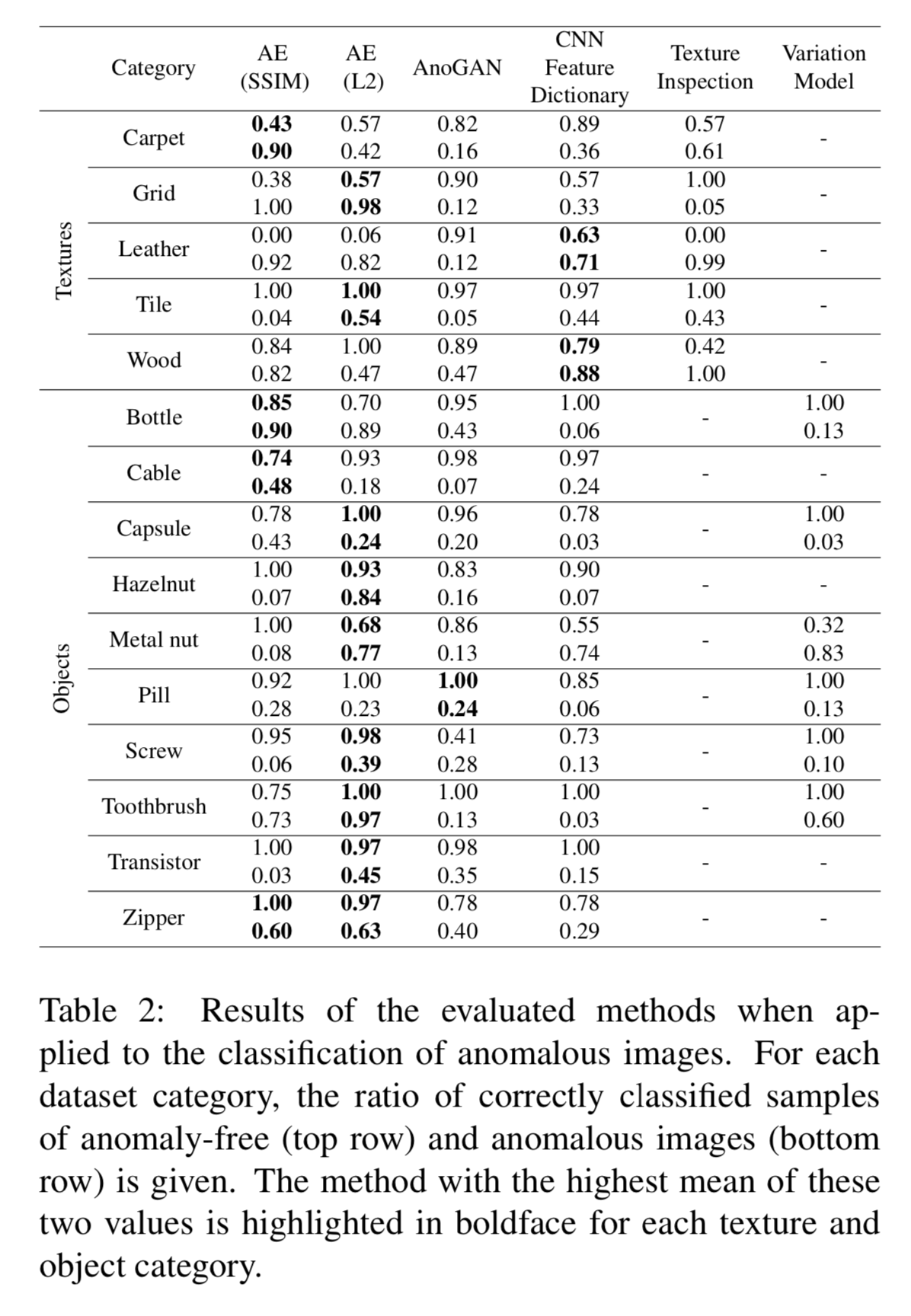
Alright - now all we need to do is pick an approach, and we’re off to the races. As we can see in figure 2, the authors explore 6 different methods, and the autoencoders (AE) perform the best on average. Autoencoders are one of the most mature unsupervised technique in deep learning for computer vision, and as we see here, can offer very respectable performance.

Today we’ll explore a newer approach to anomaly detection - Generative Adversarial Networks (GANs). GANs use a super interesting training mechanism where two neural networks compete in a game to improve overall performance, and although GANs do not deliver the top performance of the methods we see here, GANs are a hot research topic these days, and performance is quickly increasing, meaning that that figure 2 may look quite different in a few years.

The Data

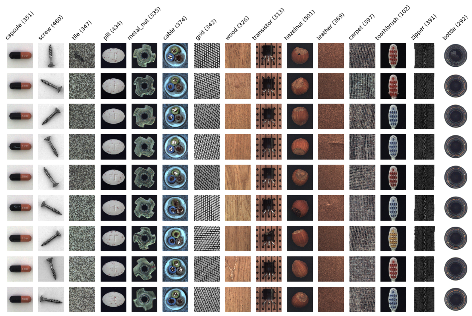
Before we start training our GAN, let’s have a quick look at our data. As you can see in figure 1, the MVTec dataset includes examples from Y different types of products. For each product type, the dataset includes a few hundred good examples, and tens of examples of different types of defects. The images are relatively high resolution, around 1000 by 1000 pixels.

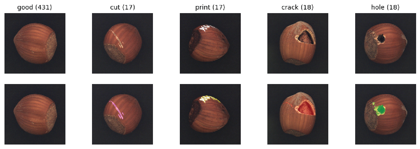
For labels, we’re given the class of each image, and a segmentation mask, as shown as colored regions in the lower portion of Figure 3. These masks indicate the location of each defect in our images.

As a deep learning practitioner working in manufacturing, I was really excited to see this dataset come out - you just don’t see public datasets like this our industry - this is really something I hope we see more of.

MLOps Questions?

The Algorithm

Alright, the fun part. It’s time to train our anomaly detection GAN. Notice in figure 2 that the MVTec paper authors don’t just use any GAN, they use an approach called AnoGAN. AnoGAN comes from a terrific 2017 paper focused on identifying anomalies in medical imagery.

If you read the AnoGAN paper, you’ll see in section 3 that the authors begin by training a DCGAN. Taking our paper inception on step deeper , DCGAN refers to an important 2016 paper by Alec Radford, Luke Metz, and Soumith Chintala.

Now, we should pause and point out here that traditional GANs like DCGAN really have nothing to do with anomaly detection. The GAN technique was invented by Ian Goodfellow in 2014 as a way to create realistic fake data. The key insight of the AnoGAN paper is a technique for using GANs to perform anomaly detection. With this in mind, let’s dive into GANs, and once we have a trained GAN in hand, we’ll zoom back out and use the AnoGAN approach with our trained GAN to fine anomalies.

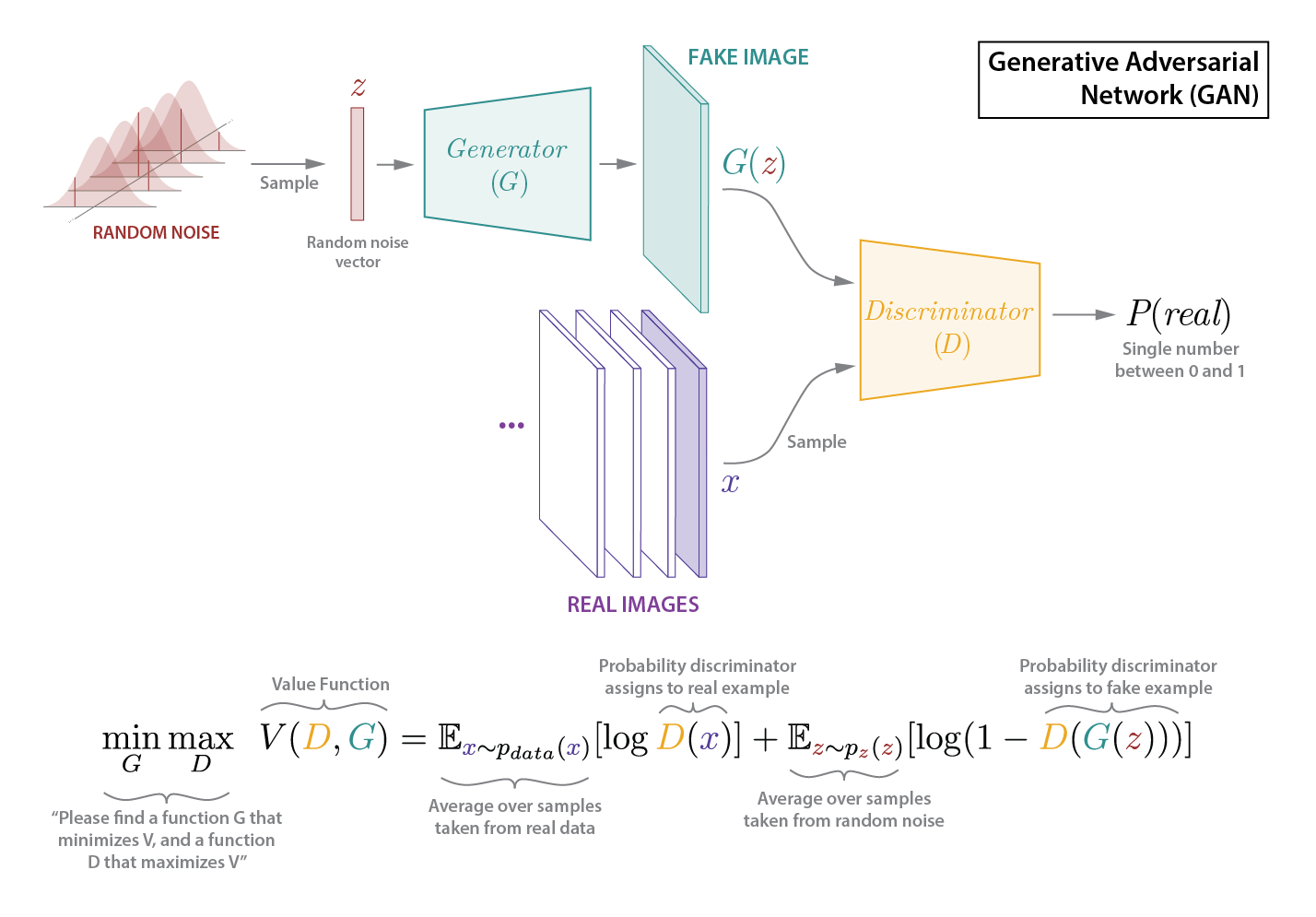
Figure 4 shows how GANs are built. Unlike traditional supervised approaches, or unsupervised approaches like autoencoders, GANs use two separate neural networks - one called a generator (G in figure 4) and one called a discriminator (D in figure 4). The discriminator very similar to traditional image classification neural networks - it takes in an image and predicts a discrete class. However, our discriminator has a simpler job than a traditional image classifier - instead of predicting the class of the image (e.g. cat, dog, bicycle, chicken…), the discriminator’s job is to determine if its input image belongs to just one of two classes: real or fake.

Our generator neural network looks a bit different than most traditional deep neural networks. The biggest difference is that our generator outputs a full image, not a discrete class. The generator’s job is to take a relatively small vector (length 100 in DCGAN) and generate a fake image from this vector. In practice researches mostly just use random values for this vector during training. That may sound a bit weird (because it is), but don’t let this randomness fool you - although the vectors are chosen randomly during training - the fact that they are low dimensional (compared to our images) means that our generator will effectively learning a transformation from a low dimensional “latent” space to the high-dimensional space of images of good products - this mapping will be critical later, as the low dimensional latent space represented a manifold of good products in a higher dimensional space of all other images, including bad products - cool, right? We’re getting a bit ahead of ourselves though, lets discuss how these pieces fit together to create a GAN.

So we have to two neural networks, one that’s supposed to learn to generate fake images, and not that’s supposed to learn to differentiate real from fake images.

Now, how do we train these suckers?

This is where GANs get really clever. To train our GAN we have our two networks play a game. We keep score in this game using a value function, as shown in figure 4. The value function is just a way to measure how well each network is doing. The first term of our value function, $E(log(D(x)))..$ captures how well our discriminator is able to correctly classify real data $x$ as real. The second term of our value function, $E(log(1-D(G(x)))$ captures the dynamic between our generator and discriminator. Larger values of this function correspond to our Discriminator doing well (correctly classifying fake images and fake), and smaller values correspond to our generator doing well (fooling our discriminator into classifying fake images as real).

Adding our two terms together, a large overall V means that our discriminator is doing well, and a small overall V means that our generator is doing well. This function is how we keep score, and is the objective that drives our optimization.

The trick then is to train our generator to minimize V and our discriminator to maximize V - at the same time. There’s some interesting theory behind all of this that Goodfellow lays out in his original 2014 paper - in a way-too-oversimplified nutshell: by making some simplifying assumptions we can show that this GAN framework will achieve a Nash Equilibrium - where any change for a given players strategy will result in a worse outcome for that player - and in theory, this will result in identical probability distributions between our real and fake data, making for fake images that are indistinguishable from real data. The theory is really interesting, I recommend checking out Goodfellow’s original paper , and outstanding book on deep learning for more information.

Now, as interesting as the theory behind GANs is, just like much of deep learning, the practical state-of-the arts is significantly ahead of any theoretical understanding. The assumptions required to achieve Nash Equilibrium can not be implemented in practice, and the best theory can really do today is act as a guide for experimentation.

With this in mind, let’s press forward with implementing and training DCGAN. We'll pick up in a Jupyter Notebook start by implementing the DCGAN archtecture (figure 5, below) in pytorch.

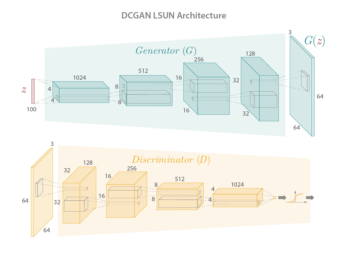
Jupyter Notebook to Implement the DCGAN Architecture

In the embedded notebook below we begin implementing the DCGAN archtecture (figure 5, above) in pytorch.

Note: the embedded notebook below is just a render. If you want to take the notebook for a live spin, check out the live Jupyter notebook on Google Colab.

Summary

In this article we showed the reader how to train a Generative Adversarial Network (GAN) on a manufacturing dataset. We created an anomaly detection algorithm using our trained GAN, and explored its performance.

If you'd like to know more about how you can use GPUs to accelerate GAN training, check out our AI Accelerator Package with ePlus and NVIDIA. It can help your organization save up to 85% on its cloud GPU bill -- check out the AI Accelerator Package homepage to download the cost study eBook.

If you'd like to know more about putting ML applications such as GANS into production with MLOps, check out our latest book with O'Reilly, "Kubeflow Operations Guide".

If you want to run a quick variation on your AWS Cloud GPU costs, check out our online GPU cost calculator.